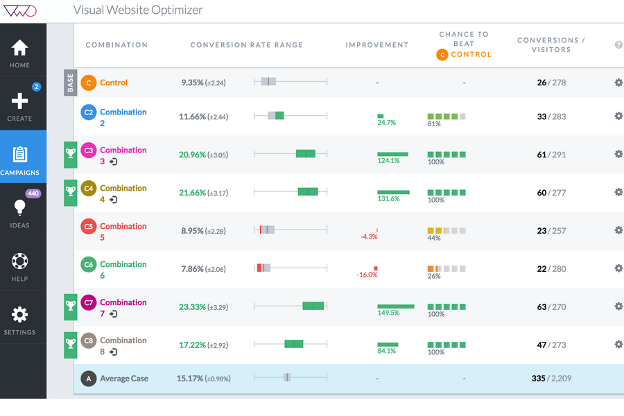
Have you wondered how to design and run online experiments? In particular, how to implement an experiment dashboard such as the one enpictured below (in this case Visual Website Optimizer) and how to use this in your product? Good, lets have a quick look!

On a pure technicall side, the first thing we have to implement is a way to define an experiment as a set of variables we want to try out and a value mapping for the audience. The most important part here is that, for a signle user, the assignment should be the same for a single experiment, e.g., the user is always in the same of two groups. However, it should different across the experiments. The latter is known as a carry-over error, and it is for example if the same user is assigned to the same test group across different experiments.

Facebook has previously released PlanOut, a platform for Online field experiments. Apart from the language itself, the essense of this project is in the random.py which demonstrates a possible way of mapping users or pages to the random aleternatives. In short, each experiment and variable has a salt to be added on top of the user or page id hash to enforce randomization across experiments and variables. The resulting hash is then mapped to the final value through modulo arithmetic and a set of linear transformations. Given this, it is fairly easy to design an API or a library to represent an experiment with a variety of options and to assign those to users in a controlled and consistent fashion. Or you can just use PlanOut or VWO right out of the box.

Settled with the setup and random assignment parts, the next question is how to actually design and run an experiment for your needs. For this, I highly recomment to take a quick look at the original paper describing PlanOut and its presentation, as well as a nice presentation  and a great tutorial about implementing and analysing online experiments at Facebook. Furthermore, there is a series of interesting publications from Microsoft (a survey, a paper and another paper) explaining numerous caveats of running controlled experiments on the web. In particular it explains statistical significance, power, and several types of mistakes it is possible to run into.

If resarch papers sound just too dry and formal, there are several interesting guides explaining A/B testing and its pitfalls in a very accessible manner:

• A/B tests. How to make it reasonable (Edrone)
• The ultimate guid to A/B testing (Unbounce)
• Why Every Internet Marketer Should Be a Statistician (Analytics Toolkit)
• Type 1 and 2 errors, and how large should your A/B test sample size be (Visual Website Optimizer) 

Finally, when it comes to presenting and interpreting the results, this A/B test analysis tool provides a simple view similar to the one in the screenshot above. Otherwise, there are several online calculators for various computations that do not require a PhD in statistics - sample size, experiment duration,comparing two rates (chi-squared test), comparing two series (t-test).

Have fun!

In the previous posts I have mentioned using Scikit-Learn, gRPC, Mesos and Prometheus. In the following, I would like to tell how all these components can be used to build a classification service and my experience with running it in a relatively large production system. For practical reasons I omit most of the actual code, and instead describe the important parts of the server script and give a reference to the external documentation when necessary.

THE PROBLEM

As a part of our daily operation at Cxense we crawl millions of Web-pages and extract their content including named entities, keywords, annotations, etc. As a part of this process we automatically detect language, page type, sentiment, main topics, etc. Skipping the details, in the following we implement yet another text classifier using Scikit-Learn.

As most of our system is implemented in Java, also including the crawler, we implement this classifier as a micro-service. For some documents therefore, the crawler will call our service, providing page title, url, text, language code and some additional information and in return retrieve a list of class names and their approximate probabilities. We further use an absolute time limit of 100 ms (end-to-end) for the classification task.

THE SOLUTION

For classification itself we use a simple two-stage pipeline, consisting of a TfidfVectorizer and a OneVsRestClassifier using LinearSVC. A separate model is trained for each of the several supported languages, serialized and distributed on the deployment. In order to communicate with our service, we use gRPC, where we define the protocol in the proto3 format and compiled it for both Java (the client) and Python (the server):

syntax = "proto3";

service Classifier {
    rpc Classify(Document) returns (Classification) {}
}

message Document {
    string url = 1;
    string title = 2;
    string text = 3;
    Language lang = 4;
    ...
}

message Classification {
    repeated Class classes = 1;
    message Class {
        string name = 1;
        float prob = 2;
    }
}

Next we implement a simple servicer, which invokes the classifier for a given language with the remaining request fields and return the classification results (class names and scores) wrapped in a response object:

...
class ClassifierServicer(proto_grpc.ClassifierServicer):

    def __init__(self):
        self.models = ...
        
    def Classify(self, request, context):
        url = request.url
        title = request.title
        text = request.text
        lang = proto.Document.Language.Name(request.lang)
        results = self.models[lang].classify(url, title, text)
        return proto.Classification(
            [proto.Classification.Class(name, prob) for name, prob in results])

To measure classification latency and the number of exceptions we further add a number of Prometheus metrics and annotate the classification method:

...
class ClassifierServicer(proto_grpc.ClassifierServicer): 
    ...
    REQUEST_LATENCY = Histogram('clf_latency_seconds', 'Request latency in seconds')
    REQUEST_ERROR_COUNTER = Counter('clf_failures', 'Number of failed requests')

    ...
    @REQUEST_LATENCY.time()
    @REQUEST_ERROR_COUNTER.count_exceptions()
    def Classify(self, request, context): 
        ...

To log the classification requests and results we add a queue to the servicer and write serialized JSON objects to it on request. We also implement a scheduled thread that drains the queue and writes the strings to disk:

...
     def __init__(self):
        ...
    	self.log_queue = queue.Queue()

   	def Classify(self, request, context): 
    	...
    	self.log_queue.put(json.dumps({'url': url, 'title': title, 'text': text, 'language': lang, 'classification': dict(results)}))
    
    def log_requests(self):
        # Drain the queue:
        requests = []
        while not self.log_queue.empty():
            requests.append(self.log_queue.get())
    
        # Write to file:
        if requests:
            filename = datetime.now().strftime('./request-%Y-%m-%dT%H.log')
            with open(filename, 'a', encoding='utf_8') as f:
                for request in requests:
                    f.write(request + '\n')
    
        # Repeat every second:
        t = threading.Timer(1, self.log_requests)
        t.daemon = True
        t.start()

The reason for doing this is that we want to avoid waiting for disk I/O on the classification requests. In fact this trick dramatically improves the observed latency on the machines with heavy I/O load and bursty requests.

Further we customize the HTTP server used by Prometheus client to return metrics on /metrics path (used for metric collection), “status”:”OK” on /status (used for health checks) and 404 otherwise:

...
def start_http_server(port):
    class HttpRequestHandler(BaseHTTPRequestHandler):
        def do_GET(self):
            if self.path == '/status':
                self.send_response(200)
                self.send_header('Content-type', 'text/plain; charset=utf-8')
                self.end_headers()
                self.wfile.write(bytes('{"status": "ok"}', 'utf-8'))
            elif self.path == '/metrics':
                self.send_response(200)
                self.send_header('Content-type', CONTENT_TYPE_LATEST)
                self.end_headers()
                self.wfile.write(generate_latest(core.REGISTRY))
            else:
                self.send_error(404)
    
        def log_message(self, format, *args):
            return
    
    class HttpRequestServer(threading.Thread):
        def run(self):
            httpd = HTTPServer(('', port), HttpRequestHandler)
            httpd.serve_forever()
    
    t = HttpRequestServer()
    t.daemon = True
    t.start()

Now, we implement the server itself as a thread taking two ports as arguments. The http port is used for health checks and metric collection and the grpc port is used for classification requests. For the http port we will use the number supplied by Aurora (see below) and for the gprc port we use port 0 to get whatever is available. To know which ports were allocated we write both to a JSON file:

...
class ModelServer(threading.Thread):

    def __init__(self, http_port, grpc_port=0):
        super(ModelServer, self).__init__()
        self._http_port = http_port
        self._grpc_port = grpc_port
        self._classifier = ClassifierServicer()
        self._stopper = threading.Event()
    
    def stop(self):
        self._stopper.set()
    
    def stopped(self):
        return self._stopper.isSet()
    
    def run(self):
        self._classifier.log_requests()
    
        grpc_server = grpc.server(futures.ThreadPoolExecutor(max_workers=8))
        proto_grpc.add_ClassifierServicer_to_server(self._classifier, grpc_server)
        self._grpc_port = grpc_server.add_insecure_port('[::]:%s' % self._grpc_port)
        grpc_server.start()
    
        start_http_server(self._http_port)
    
        service_info = json.dumps({'services': [
                {'service': 'clf-grpc', 'port': self._grpc_port},
                {'service': 'clf-health', 'port': self._http_port}]})
        print_and_flush(service_info)
    
        with open('./service.json', 'w', encoding='utf-8') as f:
            f.write(service_info)
    
        try:
            while not self.stopped():
                time.sleep(1)
        except KeyboardInterrupt:
            print_and_flush("halting...")
        finally:
            grpc_server.stop(0)

def print_and_flush(s):
    print(s)
    sys.stdout.flush()

if __name__ == '__main__':
    print_and_flush('loading...')
    ModelServer(http_port=int(sys.argv[1])).start()

Threading logic herein allows us quite simple unit test usage, for example:

...
class TestAll(unittest.TestCase):

    @classmethod
    def setUpClass(cls):
        ...
        # Build and serialize test models.
        for language in [...]:
            train_model(language)
    
        # Start the server, give it some time.
        cls.server = ModelServer(http_port=12345)
        cls.server.start()
        time.sleep(1)
    
    def test_basics(self):
        address = 'localhost:%s' % TestAll.server._grpc_port
        result = classify(address, ...)
        self.assert...
       
    @classmethod
    def tearDownClass(cls):
        # Stop the server, give it some time.
        cls.server.stop()
        time.sleep(1)
    
        # Delete temporary files.
        os.remove('service.json')
        for logfile in glob('request-*.log'):
            os.remove(logfile)

if __name__ == '__main__':
	unittest.main()

Further, we provide Aurora configuration that consists of the following tasks:

1. Fetch code and data from into the sandbox.
2. Activate virtual environment and start the server using thermos.ports[http]
3. Wait for service.json to be written and register clf-health and clf-grpc in the consulate. Use clf-health for httpcheck.
4. On shutdown, deregister the service in consulate.
5. Otherwise, delete request logs that are more than 12 hours old.

fetch_all = ...

run_server = Process(
  name = 'run_server',
  cmdline = 'source venv/bin/activate && venv/bin/python server.py ')

register_service = Process(
    name = 'register_service',
    cmdline = 'HTTP=$(service-file-get clf-health service.json 300); \
        GRPC=$(service-file-get clf-grpc service.json 0); \
        consulate register clf-health -s clf-health -a $(hostname) -p $HTTP httpcheck 10 http://localhost:$HTTP/status; \
        consulate register clf-grpc -s clf-grpc -a $(hostname) -p $GRPC httpcheck 10 http://localhost:$HTTP/status')

deregister_service = Process(
    name = 'deregister_service',
    final = True,
    cmdline = '/usr/local/bin/consulate deregister clf-health; \
        /usr/local/bin/consulate deregister clf-grpc; sleep 5')

log_removal = Process(name = 'log_removal', cmdline = 'while true; do find . -name request\*.log -mmin +720 -print0 | xargs -0 --no-run-if-empty rm; sleep 3600; done')

server_task = SequentialTask(processes = [fetch_all, run_server], resources = Resources(cpu=1, ram=4*GB, disk=3*GB))
register_task = Task(processes=[register_service], resources=Resources(cpu=0.01, ram=0.1*MB, disk=1*MB))
deregister_task = Task(processes=[deregister_service], resources=Resources(cpu=0.01, ram=0.1*MB, disk=1*MB))
log_removal = Task(processes=[log_removal], resources=Resources(cpu=0.01, ram=0.1*MB, disk=1*MB))

jobs = []
for dc in [...]:
  jobs.append(Service(cluster = dc,
          environment = 'prod',
          tier = 'preferred',
          role = ...,
          name = 'clf',
          update_config = UpdateConfig(watch_secs = 300, batch_size = 1),
          task = Tasks.combine(server_task, register_task, deregister_task, log_removal),
          constraints = {'host': 'limit:1'},
          instances = 4))

Note that here we use four instances per data center, each requires slightly more than 1 CPU, 4GB RAM, 3GB disk. We also restrict our job to have no more than one instance per host

From here we can start, stop, update and scale our jobs using Aurora’s client commands. Beyond what is mentioned we implement classification service client in Java and embed it into the crawler. Cxense codebase includes code for automatic resolve of clf-grpc to a list of healthy servers, and even scheduling up to 3 retries with 20 ms between and final time-out at 100ms. Here we also use Prometheus to monitor client latency, number of failed requests, etc. Moreover, we configure metric export from both clients and service, set up a number of service alerts (on inactivity, too long latency or high error rate) and Grafana dashboards (one for each DC).

THE EXPERIENCE

Initially I was quite skeptical about using Python/Scikit-Learn in production. My suspicions “were confirmed” by a few obstacles:

1. The gRPC threads above are bound to one CPU and it is really hard to do anything about that in Python. However, this is not a big deal as we can scale by instances instead of cores. In fact, it is better.
2. Ocasionally tasks get assigned to “slow” nodes which makes 90+ percentile latency higher in orders of magnitude. After some investigation with colleagues, we found that this may happen on I/O overloaded nodes. Delayed logging demonstrated above gave us a dramatic improvement here, so it wasn’t that much of issue anymore. Otherwise, we could add a supervisor to restart unlucky jobs.
3. Grpc address lookup makes client-observed latency significantly worse than the clasification port itself. However, our codebase implements a short-term address cache, and for cached addresses the latency increase is not a big deal. The problem we have seen initially was that with a large number of crawlers and relatively small fraction of classification requests, the cold-cache chance is quite high. With increasing number of requests however, the chance of this goes down and the latency goes down as well.
4. We have observed that for bursty traffic latency jitter can be quite high and the first few requsts after a pause are likely to be out-of-time. For the client, I assume it is because of the cost of loading models back into memory and CPU caches. For the server, I assume it is becauce of the closed connections and cold address caches. The funny part here was that this issue is less with increased number of requests. In fact, we have seen latency (both for the client and the server) go down after doubling the number of requests by adding support for a new language without increasing the total resource budget (CPU, RAM, disk).

So in total, the experience in prod was quite postive. Apart from the points mentioned above, there were no problems or accidents and I have not seen any server-side exceptions. The only time I had to find why the classifier was suddenly inactive was when AWS S3 went AWOL and broke the Internet.

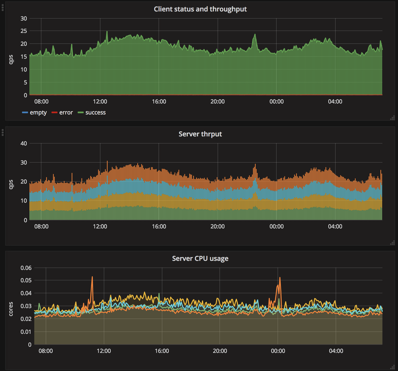
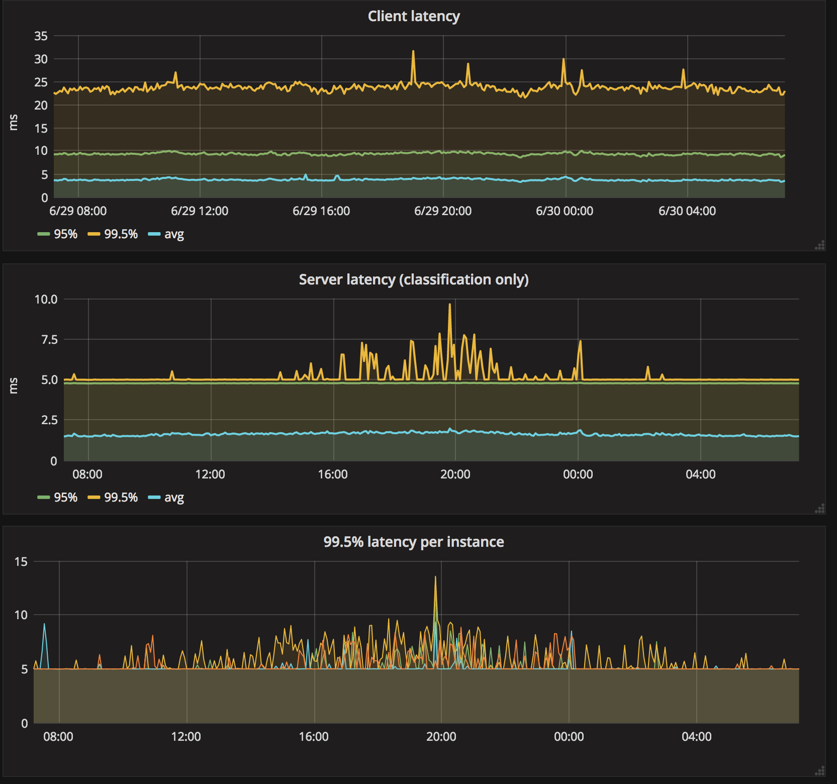
On the final note, here is a dashboard illustrating the performance on production traffic in one of our datacenters (the legend was removed from some of the charts).

A year ago I wrote a post about the things I have learned during my PhD at NTNU. Since then I wanted to write about my experience as a Software Engineer at Cxense. I am sure that the list of what I have learned over the past four and half years would be very long, so instead I would like to summarize it as the five best things about working at Cxense. So here it goes:

Challenges

Engineers love tough problems and here are plenty of them. Within a month after starting at Cxense, I have been thrown into designing a weighting function that would include dwell time and page popularity into computing the impact of the page’s content on a user’s interest profile and implementing complex filters for a distributed low-level database (solved by implementing bit-wise logical filters and a stack machine). At the same time I reviewed a highly impressive implementation for an incremental inverted index on top of a compressed integer list and lots of mind-numbing bit-twiddling code. The author was Erik Gorset, whom I am deeply grateful for all the inspiration and advice over the years. Since then my colleagues and I have worked on thousands of dazzling problems within areas of distributed databases, data mining, machine learning and development operations, not to mention all bugfixes. Fixing bugs is actually fun, because it feels good to trace that flaw by the end of the day and fix it. Nothing is perfect, and that is also why you need to write good unit and integration tests. Writing tests is hard and time consuming, but it always pays off in the long run. Code reviews provide a great opportunity to learn how other people think and tackle challenges, both for the reviewer and the one being reviewed.

Scale

When I met guys from Cxense for the first time five years ago, they were going live with a large publisher network in Spain. I remember seeing a live chart with the event traffic instantly increasing ten times or so. The guys were very excited about whether the system would handle the challenge, and it did. Since then the numbers have increased by many orders of magnitude. We passed the 20 billion page views per month mark a two years ago. Counting all possible type of events we collect that would be above 60 billion events per month or more than one terabyte of data per day. Crawling is also approaching 100 million Web pages per month these days. These numbers are huge, but the transition impresses me even more because it is impossible to design a system for this kind of growth. A solution that is sufficient at one point has to be phased with a better solution at another point, which in its turn will become obsolete at a later point. Nevertheless, despite this tremendous growth we are still able to serve real-time data with latency counted in just milliseconds.

Tools

We used Java since the beginning, and previously most of us used Eclipse with a common setup for CheckStyle and FindBugs. Nowadays, the majority is using IDEA, but we still heavily rely on a common code style, static checks and a set of best practices. We use git with a common code repo and another repo for data center configuration related stuff. At the moment we use GitLab for code reviews and a homemade builder doing speculative merge builds and lots of awesomeness like stability tests and automatic deployment to the staging environment. Skipping the details, what I love most is that we can deploy anything within just a few minutes even at the current scale.

Initially we would rent hardware and run things on bare Ubuntu servers ourselves, using Upstart for continuous services and crontab for scheduled tasks. The implementation would be in Java with a BASH or Python wrapping and most of the internal services would often have a fixed HTTP port with JSON input/output. Data pipelines would often be implemented with a few simple of components, one of which would for example receive data and write it to disk using atomic appends, while another would tail the written data and crunch it or send it to another service (again using JSON over HTTP). This gave us many nice benefits for scaling (add more consumers behind a load balancer), failover (as long the data is written to disk somewhere, nothing is lost), debugging (just look up the logs) and monitoring.

With the growth mentioned earlier, we are now moving over to Mesos (running on top of our own hardware) and running things with Aurora. Nowadays, we use gRPC for communication between services, Consul for service discovery, Prometheus for performance metrics and alerting and Grafana for monitoring dashboards. Things are getting even better and deployments across multiple data centers and hundreds of machines are still within minutes. In fact, they are only getting faster.

Flow

When I started at Cxense, it was a typical startup – we used JIRA for issue tracking, but it was a mix of roadmap features, devs’ own ideas and FIXMEs, support issues reported by customers or deliverables promised by sales guys, with no clear definition for priorities or deadlines. We would pick tickets that we thought were most urgent or important and did our best to solve them most efficiently. We would discuss this in daily standups and perhaps present some cool new features at regular video calls. Once in a while each developer would have a hell week, when he or she would be facing all the incoming support issues, chats and alerts. The fun part in this was that one could hack a set of new features over a weekend or handle a hundred of support issues during a hell week. The boring part of this was figuring out where the company was going after all.

Today everything is much more organized. For the feature part, we have a roadmap for a year ahead, which then drains down to specific plan for each quarter for each team. For the support part, we have several lines of highly trained professionals, which filter out all the noise and leave only actual issues to be fixed. For most teams, we run two-week iterations, where tickets come from the development roadmap for the given quarter, pre-triaged support issues meeting the bar, or the technical roadmap issues. The last part covers things like scalability improvements, shifting out components with better alternatives, or making the system more resilient. We separated on-call incidents from the rest of the JIRA issues long time ago, but for the last year or so we have also been working on growing a highly skilled infrastructure team.

Each iteration starts with a planning phase involving team leads and engineering managers, followed by a meeting where team members are free to pick the issues they like to put their hands on and with respect to the amount of work they can handle in the next sprint. The sprint ends with a highlight of the most important things a team has achieved and a demonstration of the most interesting features.

People

The most important ingredient in a great workplace is people. Joining Cxense I had no expectations other that here would be the best people in the industry. This turned out to be true, and I am lucky to be working with some of the best engineers and business experts in the field. It is a pleasure to be a part of the discussions and changes we have done over the years and those to come.

Cxense is spread across 5 out of the 7 parts of world. Therefore, it is quite common that my day would start with a quick fix for a support issue from Tokyo, followed by a few quick answers to questions from my colleagues in Samara, Munich, Buenos Aires or San Francisco. The changes I made the day before would be reviewed by a colleague sitting next to me in Oslo and then distributed to the data centers across the world. After the lunch I would focus on the next feature, working with the data from a major news publisher in USA, Argentina, Norway or Japan. On the way home, I would comment on the global company chat and receive a funny cat picture from a colleague in Melbourne. The world is very small when it comes to Cxense.

In conclusion

Cxense grew a lot over the years I have been working here, but it remains a fast-paced company with talented people, exciting challenges and a cool software stack. Things are getting better and I can only imagine where we will be in the next five years. While working here I have learned a billion things about software development (and yet still learning), and I hope that this post was able to bring some of those insights to you. …ah, and by the way, we are hiring!

Scikit-Learn is a great library to start machine learning with, because it combines a powerful API, solid documentation, and a large variety of methods with lots of different options and sensible defaults. For example, if we have a classification problem of predicting whether a sentence is about New-York, London or both, we can create a pipeline including tokenization with case folding and stop-word removal, bigram extraction, tf-idf weighting and support for multiple labels, train and apply it in merely 8 lines of code (well, excluding imports and input specification).

vec = TfidfVectorizer(ngram_range=(1, 2), stop_words='english', max_features=15)
clf = OneVsRestClassifier(LogisticRegressionCV())
pipeline = make_pipeline(vec, clf)
mlb = MultiLabelBinarizer()
y_train = mlb.fit_transform(y_train)
pipeline.fit(X_train, y_train)
predicted = pipeline.predict(X_test)
print(zip(X_test, mlb.inverse_transform(predicted)))

Furthermore, we can easily add cross-validation and parameter tuning, etc., in just a few more lines. Check out this great introductory video series for all the cool features you can use right from the beginning. But lets go back a bit! Assume we have the following training data:

[("new york is a hell of a town", ["New York"]),
 ("new york was originally dutch", ["New York"]),
 ("the big apple is great", ["New York"]),
 ("new york is also called the big apple", ["New York"]),
 ("nyc is nice", ["New York"]),
 ("people abbreviate new york city as nyc", ["New York"]),
 ("the capital of great britain is london", ["London"]),
 ("london is in the uk", ["London"]),
 ("london is in england", ["London"]),
 ("london is in great britain", ["London"]),
 ("it rains a lot in london", ["London"]),
 ("london hosts the british museum", ["London"]),
 ("new york is great and so is london", ["London", "New York"]),
 ("i like london better than new york", ["London", "New York"])]

Our model can easily predict the following:

[("nice day in nyc", ["New York"]),
 ("welcome to london", ["London']),
 ("hello simon welcome to new york. enjoy it here and london", ["London", "New York"])]

But how? Well, we know that the model’s decision function computes a dot product between the input features and the trained weights and we can actually see the computed numbers:

print(pipeline.decision_function(X_test))

[[ -7.96273351   1.04803743]
 [ 22.19686347  -1.39109585]
 [  5.48828931   1.28660432]]

So, a positive number indicates positive classification ([London, New-York]), and we can convert this to some sort of “probability” estimation:

print(np.vectorize(lambda x: 1 / (1 + exp(-x)))(pipeline.decision_function(X_test)))

[[  3.48078806e-04   7.40397853e-01]
 [  1.00000000e+00   1.99232868e-01]
 [  9.95882115e-01   7.83571880e-01]]

However, it would be nice if we could know exactly which words have contributed to the final score. And guess what, there is an awesome library to explain you this like are five years old:

import eli5
eli5.show_prediction(clf, X_test[0], vec=vec, target_names=mlb.classes_)

Note that the numbers here are exactly what we have seen above, but in addition we get a visual explanation of which words have trigged positive and negative signals. Moreover, with a bit of trickery to work around this issue, we can also dump the features computed for our model as a neatly looking heat map:

setattr(clf.estimator, 'classes_', clf.classes_)
setattr(clf.estimator, 'coef_', clf.coef_)
setattr(clf.estimator, 'intercept_', clf.intercept_)
eli5.show_weights(clf.estimator, vec=vec, target_names=mlb.classes_)

So far, working with scikit-learn and eli5 is as fun as Transformers were when I was five! And working with a relatively large dataset is just as easy as the toy example shown here in. Man, this is great, but what about using it in a production system you say? Well, lets talk about that next time ;)

Read more

Recently I have been working on a text-classification task. Along the way I have tested out three interesting machine learning frameworks which I would like to address in the next few posts. This time I start with the Apache Spark’s MLlib.

Spark got my attention quite a long time ago and it is extremely useful for data exploration tasks where you can simply put lots of data on HDFS and then use a Jupyter notebook to transform the data interactively. However, although training is preferably done offline using a large number of examples (where Spark becomes handy), the classification part is often desired to be a short-latency/high-throughput task. As the framework itself brings quite a lot of overhead, it could be nice if the API methods could be executed without the Spark cluster when necessary. In that case you could use the cluster to build a model, serialize and ship it to a worker, which will then use the model on the incoming instances.

My earlier implementation of text-classification for Reuters 21578 can be executed as a simple JAR, but as I wrote earlier, it was quite a dance to do this correctly. Moreover, in that example I have used the RDD part of the MLlib API and ended up with a very verbose Java code.

Recently, the API has been extended with pipelines and many interesting features (most likely inspired by Scikit-Learn) making it really easy to implement a classifier in just a few lines of code, for example:

labelIndexer = StringIndexer(inputCol="label_text", outputCol="label")
tokenizer = Tokenizer(inputCol="text", outputCol="tokens")
remover = StopWordsRemover(inputCol=tokenizer.getOutputCol(), outputCol="filtered")
hashingTF = HashingTF(inputCol=remover.getOutputCol(), outputCol="features")
lr = LogisticRegression(maxIter=20, regParam=0.01)
ovr = OneVsRest(classifier=lr)
pipeline = Pipeline(stages=[labelIndexer, tokenizer, remover, hashingTF, ovr])
model = pipeline.fit(train_paired)
result = model.transform(test_paired)
predictionAndLabels = result.select("prediction", "label")
evaluator = MulticlassClassificationEvaluator(metricName="accuracy")
print("Test set accuracy = " + str(evaluator.evaluate(predictionAndLabels)))

Nevertheless, this new DataFrame-based part of the API has not yet reached parity with the old RDD-based part of the API. The latter is planned to be deprecated when this happens, but currently some of the methods are available only through the old part of the API. In other words, a strong dependency between the algorithms and the underlying data structure is a real problem here. I only hope that the same will not happen again if the DataFrame concept gets replaced by a better idea in a year or two.

Finally, although there are quite many resources available online (books, courses, talks, slides, etc.), the documentation of MLlib is far from good (especially the API docs) and the customization part beyond simple examples is a nightmare (an exercise for the reader: add bigrams to the pipeline above), if possible at all. On the positive side, Spark is great for certain use cases and is being actively developed with lots of interesting features and ideas coming up next.

Read more