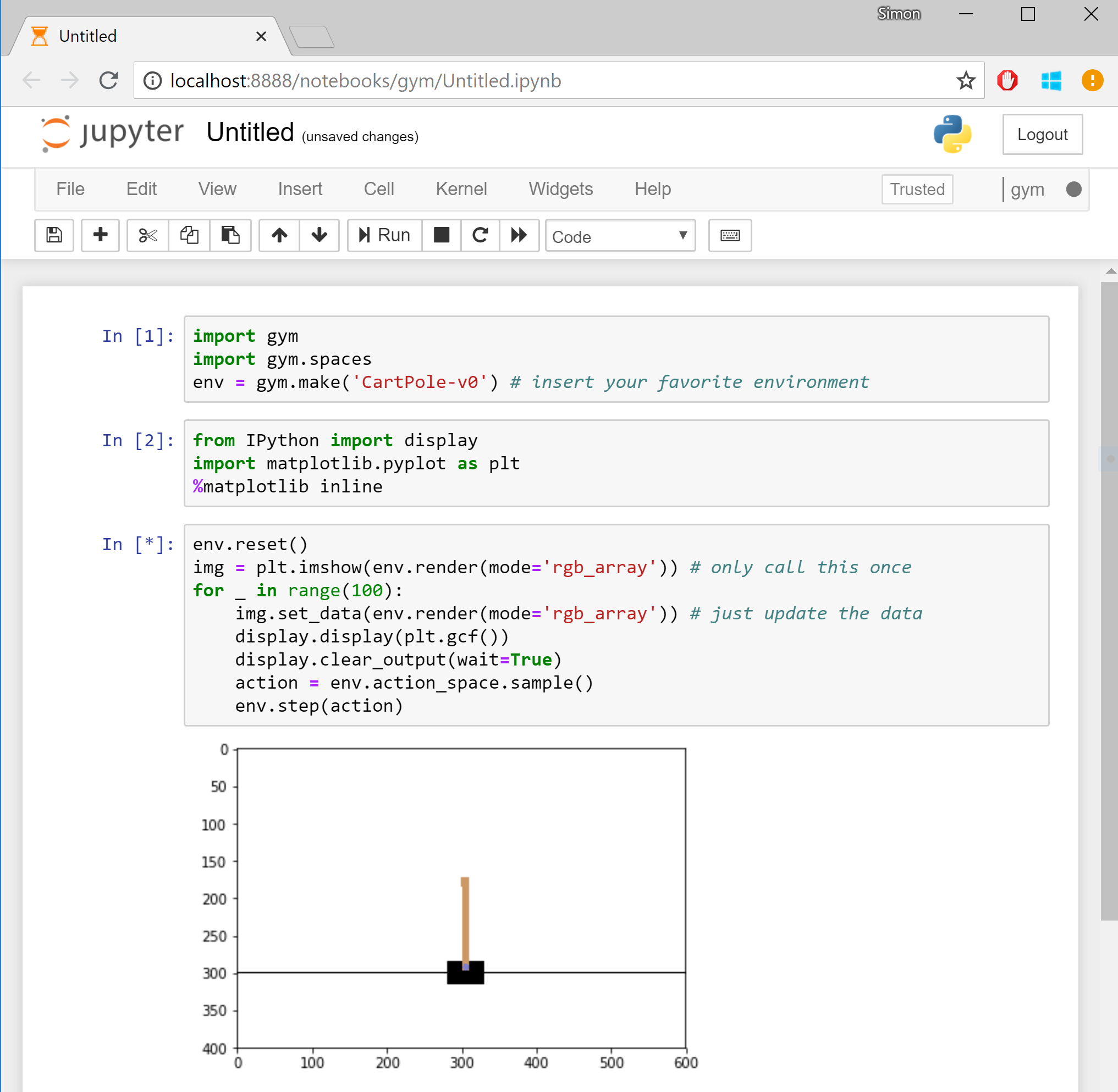
Open AI Gym is a fun toolkit for developing and comparing reinforcement learning algorithms. It provides a variety of environments ranging from classical control problems and Atari games to goal-based robot tasks. Currently it requires an amout of effort to install and run it on Windows 10. In particular you need to recursively install Windows Subsystem for Linux, Ubuntu, Anaconda, Open AI Gym and do a robot dance to render simulation back to you. To make things a bit easier later you would also like to use Jupyter Notebook. In the following you will find a brief step-by-step description as of September 2018 with the end result looking like this:

First we install the Linux subsystem by simply running the following command as Administrator in Power Shell:

Enable-WindowsOptionalFeature -Online -FeatureName Microsoft-Windows-Subsystem-Linux

After restarting the computer, install Ubuntu 18.04 from the Windows Store, launch and run system update:

sudo apt-get update
sudo apt-get upgrade

Next we install Anaconda 3 and its dependencies:

sudo apt-get install cmake zlib1g-dev xorg-dev libgtk2.0-0 python-matplotlib swig python-opengl xvfb
wget https://repo.continuum.io/archive/Anaconda3-5.2.0-Linux-x86_64.sh
chmod +x Anaconda3-5.2.0-Linux-x86_64.sh
./Anaconda3-5.2.0-Linux-x86_64.sh

Then we ensure that .bashrc file has been modified as necessary. If not, adding . /home/username/anaconda3/etc/profile.d/conda.sh at the very end should do the kick.

After this, we relaunch the terminal and create a new conda environment called gym:

conda create --name gym python=3.5
conda activate gym

and install Gym and its dependencies:

git clone https://github.com/openai/gym
cd gym
pip install -e .[all]

As we are also going to need matplotlib, we install it by running:

pip install matplotlib

Next we install jypyter notebooks and create a kernel pointing to the gym environment created in the previous step:

conda install jupyter nb_conda ipykernel
python -m ipykernel install --user --name gym

Now we run the magic command which will create a virtual X server environment and launch the notebook server:

xvfb-run -s "-screen 0 1400x900x24" ~/anaconda3/bin/jupyter-notebook --no-browser

no-browser tells that we don’t want to open a new browser in the terminal, but prompt the address. The address can now be pasted in the browser in your Windows 10, outside of the Ubuntu env.

Next we create a new notebook by choosing “New” and then “gym” (thus launching a new notebook with the kernel we created in the steps above), and writing something like this:

import gym
import 
env = gym.make('CartPole-v0')

from IPython import display
import matplotlib.pyplot as plt
%matplotlib inline

env.reset()
img = plt.imshow(env.render(mode='rgb_array')) # only call this once
for _ in range(100):
    img.set_data(env.render(mode='rgb_array')) # just update the data
    display.display(plt.gcf())
    display.clear_output(wait=True)
    action = env.action_space.sample()
    env.step(action)

This tells to create a new cart pole experiment and perform 100 iterations of doing a random action and rendering the environment to the notebook.

If you are lucky, hitting enter will display an animation of a cart pole failing to balance. Congratulations, this is your first simulation! Replace ‘CartPole-v0’ with ‘Breakout-v0’ and rerun - we are gaming! AWESOME!

Flutter is a great Google SDK allowing effortless creation of mobile apps with native interfaces on iOS and Android. To install it follow the official installation instructions. Here are a few additional tips for Mac and Windows:

• If you are using fish, add set PATH /Users/simonj/flutter/bin $PATH to your .config/fish/config.fish
• For android emulation support install Androind Studio and create a new emulated device, lets call it Pixel_2_API_26. To launch the emulator, run ~/Library/Android/sdk/tools/emulator -avd Pixel_2_API_26 on Mac or C:\Users\<name>\AppData\Local\Android\Sdk\emulator\emulator.exe -avd Pixel_2_API_26 on Windows.
• Disabling Hyper-V may help if you experience Windows crashes when running Android emulator.
• Some useful commands:
  • flutter doctor # helps to diagnose problems, install missing components, etc.
  • flutter build apk # builds apk
  • flutter install -d # installs apk to a device. to use your actual phone, mount the phone with usb debug enabled
  • flutter devices # to list devices
• To use visual studio code, follow these instructions or just run code . from your flutter terminal/project and install Flutter and Dart plugins.
• Check out awesome-flutter for example and inspiration!

In the following, I briefly show how coef_, intercept_, decision_function, predict_proba and predict are connected in case of a binary LogisticRegression model.

Assume we have trained a model like this:

>>> ...
>>> lrmodel = linear_model.LogisticRegression(C=0.1, class_weight='balanced')
>>> lrmodel.fit(X_train, y_train)

The model’s coef_ attribute represents learned feature weights (w) and intercept_ represents the bias (b). Then the decision_function is equivalent to a matrix of x · w + b:

>>> (X_test @ lrmodel.coef_[0].T + lrmodel.intercept_)[:5]
    array([-0.09915005,  0.17611527, -0.14162106, -0.03107271, -0.01813942])

>>> lrmodel.decision_function(X_test)[:5]
    array([-0.09915005,  0.17611527, -0.14162106, -0.03107271, -0.01813942])

Now, if we take sigmoid of the decision function:

>>> def sigmoid(X): return 1 / (1 + np.exp(-X))

>>> sigmoid(X_test @ lrmodel.coef_[0].T + lrmodel.intercept_)[:5]
    array([ 0.47523277,  0.54391537,  0.46465379,  0.49223245,  0.49546527])

>>> sigmoid(lrmodel.decision_function(X_test))[:5]
    array([ 0.47523277,  0.54391537,  0.46465379,  0.49223245,  0.49546527])

it will be equivalent to the output of predict_proba (each touple is probabilities for -1 and 1). We see that these numbers are exactly the second column (the positive class) here:

>>> lrmodel.predict_proba(X_test)[:5]
    array([[ 0.52476723,  0.47523277],
           [ 0.45608463,  0.54391537],
           [ 0.53534621,  0.46465379],
           [ 0.50776755,  0.49223245],
           [ 0.50453473,  0.49546527]])

Finally, the predict function:

>>> lrmodel.predict(X_test)[:5]
    array([-1,  1, -1, -1, -1], dtype=int64)

is eqivalent to:

>>> [-1 if np.argmax(p) == 0 else 1 for p in lrmodel.predict_proba(X_test)] [:5]
    [-1, 1, -1, -1, -1]

which in our case is:

>>> [1 if p[1] > 0.5 else -1 for p in lrmodel.predict_proba(X_test)] [:5]
    [-1, 1, -1, -1, -1]